

Block I · Foundations of Knowledge & Reasoning · Day 006 / 180
Statistics & the Art of Not Fooling Yourself
Given enough defensible choices, many datasets contain a path to p < .05. The whole discipline is the struggle not to walk it by accident.
In 2011 three psychologists set out to prove something impossible. They sat twenty undergraduates down, played half of them the Beatles’ “When I’m Sixty-Four” and the other half a control tune, then asked a battery of questions — including each person’s date of birth. After a perfectly ordinary statistical analysis, they announced their finding: listening to “When I’m Sixty-Four” made people a year and a half younger. Not feel younger. Be younger — their birth dates said so, at .
This is, of course, impossible. A song cannot reach back and edit the year you were born. And that was exactly the point. Joseph Simmons, Leif Nelson, and Uri Simonsohn had used only standard, respectable tools, made only choices that any working scientist makes every week — and produced a statistically significant impossibility. Their paper was a deliberately absurd demonstration designed to expose a vulnerability. Today we learn what it exposed, and how a science learns to stop fooling itself.
Where we are
On Day 2 we met the replication crisis as a set of bruising numbers (97% of original psychology studies reported significant effects; only 36% replicated) and named p-hacking without yet opening it up. Today we open it up. This is the statistical engine room beneath that crisis — and beneath Day 1’s Gettier worry (a belief that’s true by luck, not connection) scaled up to entire literatures. We’ll lean hard on Day 4’s lesson that a -value is not the probability the null is true (that confusion is the base-rate fallacy in disguise), and on Day 5’s warning that which variables you control for is itself a fork in the road. Threads today: information (signal vs noise) and computation (the lab as a fallible inference machine), with a quiet preview of emergence — science as an error-correcting system bigger than any one analyst.
The hook
The easiest person to fool
“The first principle is that you must not fool yourself — and you are the easiest person to fool.” — Richard Feynman, Caltech commencement, 1974

Richard Feynman at a blackboard in 1959. The quote above comes from his 1974 Caltech commencement address on “cargo cult science.”
Feynman was talking about a kind of integrity that no formula can supply. The cruel twist of modern statistics is that the formulas can still be correct, but after flexible searching they no longer protect the nominal error rate. They lend the warm authority of mathematics to whatever you were already hoping to find.
The villain has a clinical name: researcher degrees of freedom. Every real analysis hides dozens of small, defensible decisions. Which outliers to exclude? Should you control for age? Sex? Both? Do you stop collecting data now, or run twenty more participants? You measured three outcomes — which do you report? Each choice, taken alone, is innocent. Taken together, made after you’ve glanced at how the numbers are leaning, they become a machine for minting false discoveries.
Simmons, Nelson & Simonsohn proved this with arithmetic before they proved it with the Beatles. By simulation, they showed that bundling just four ordinary degrees of freedom — peeking at the data and adding more if needed; choosing between two related outcome measures; splitting the sample by a variable like gender; dropping one of three experimental conditions — can inflate your chance of a false positive from the advertised 5% to as high as 61%. Flip enough innocent switches and a coin-flip’s worth of noise becomes a near-certainty of “success.”
Run the false-positive factory: every simulated study has no true effect, so any apparent discovery comes from the choices you permit. Watch analytic freedom turn noise into a headline.
The cases show how each analytic freedom gives pure noise another route to masquerade as a discovery.
Interactive · live Monte-Carlo simulation
The False-Positive Factory
Each run simulates ~1,500 experiments in which there is no real effect at all — two groups drawn from the same distribution. If the null is true, the model assumptions hold, and you run one pre-specified test, about 5% will still cross by chance. Now hand yourself some researcher degrees of freedom and re-run. The factory simply reports the prettiest result it can find among the analyses you've allowed.
The False-Positive Factory
Each ordinary analytic freedom multiplies the number of chances to report a chance result.
| Analytic freedom | What changes | Why it inflates false positives |
|---|---|---|
| Two outcome measures | Measure two related results and report the one that works. | Noise gets two chances to cross . |
| Optional stopping | Peek at n=20, then add participants if needed. | The stopping rule itself becomes another path through the data. |
| Flexible subgroup analysis | Try the overall result and subgroup splits. | Legitimate subgroup checks become multiple comparisons when chosen after seeing the data. |
| Drop a condition | Run three groups, then report the best pair. | The reported contrast is selected because it looks best. |
Simmons, Nelson, and Simonsohn showed that combining four such freedoms can raise a nominal 5% false-positive rate to about 61% even when the data contain no real effect.
The core model
What a -value actually says (and the six lies people tell about it)
To not be fooled, you have to know precisely what the instrument reports. Many readers, including trained scientists and a worrying number of the statistics instructors teaching them, get this wrong. So, carefully:
Definition · the p-value
The p-value is the probability — computed under a specified null model, including the null hypothesis and its sampling and modeling assumptions — that the chosen test statistic would be at least as extreme as its observed value.
Concrete version: suppose the null model says two groups have the same mean. If a difference this large or larger would occur 3% of the time under that model, then . That is not a 3% chance the null is true.
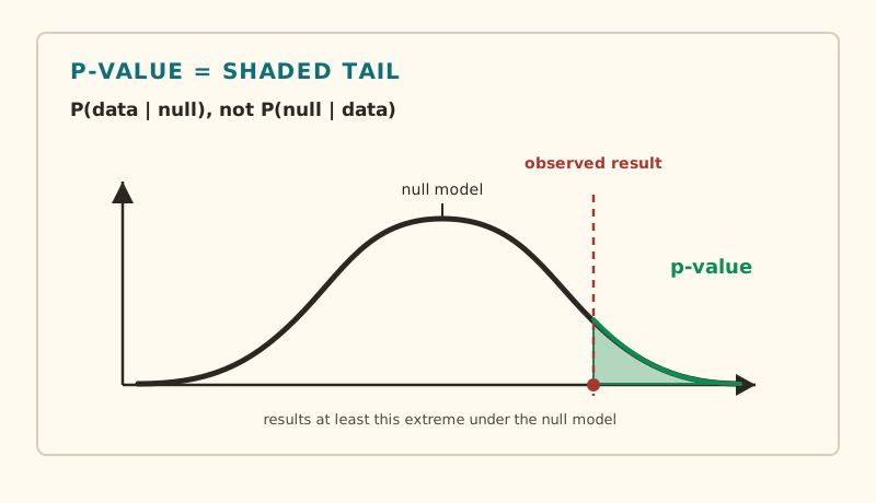
The shaded tail is the p-value: under the null model, the probability of test-statistic values this extreme or more extreme.
Read it twice. It is a tail-area statement about a chosen test statistic under the null model — schematically, . It is emphatically not a statement about the hypothesis given the data, . Confusing those two is the exact inversion Day 4 warned about with the disease-test problem: is not , and no amount of staring turns one into the other without a prior. Here are the six misreadings to burn out of your reflexes — drawn from Greenland and colleagues’ field guide to twenty-five of them:
Three probabilities people confuse
Alpha is the long-run Type I error rate of a testing procedure if the null model is true: with , about 5% of true-null tests will falsely cross the line. The false discovery rate asks a different question: over repeated use of a specified discovery procedure, what is the expected proportion of false claims among those it declares significant? That depends on base rates, power, and selection, not just . A posterior probability, such as , is different again: it needs a prior. A 5% is neither a 5% false discovery rate nor a 5% chance the null is true.
- ” means there’s a 3% chance the null is true.”No. That’s — a Bayesian quantity needing a prior. The -value already assumes the null.
- ” means a 5% chance the result is just chance.”No. Chance (the null) is the very assumption the calculation is built on; it can’t also be the thing in doubt.
- ” means there is no effect.”No. Absence of evidence is not evidence of absence — an underpowered study fails to detect real effects all the time.
- ” is the probability the alternative is true.”No. Neither nor its complement is a probability about any hypothesis.
- ”p tells you the result will replicate.”No. A low from one noisy study says little about the next study.
- ”A significant result is a large or important one.”No. With a big enough sample, a trivially small effect is “significant.” Significance ≠ size ≠ importance.
That last one is the quiet killer, so it gets its own model.
Significance is not size: meet the effect size
A -value entangles effect size, noise, sample size, and model assumptions. Pour in enough participants and even a microscopic, meaningless difference crosses the line. So grown-up statistics insists on reporting the effect size separately: Cohen’s d (a difference in means measured in standard deviations) or a correlation r. Jacob Cohen offered rough labels — d ≈ 0.2 small, 0.5 medium, 0.8 large — while cheerfully admitting they were arbitrary: “Although arbitrary, the proposed conventions will be found to be reasonable by reasonable people.” The point is not the labels. The point is that a number with no effect size attached has told you almost nothing worth knowing.
Interactive · significance versus size
The Effect-Size Dial
Set a true mean difference, a per-group sample size, and a noise level. A group means one side of the two-group comparison, such as treatment versus control; n = 50 per group means 50 observations in each side, 100 total. The plot uses fixed x and y scales: mean difference from -3 to +3, and bucket frequency from repeated estimates. Finer bars show the estimate distribution; the curve is the matching sampling distribution; the horizontal bar is the 95% confidence interval on the same x scale.
Significance versus size
The same true effect can look very different as sample size and noise change.
| Scenario | p-value | 95% CI for mean difference | Cohen’s d | Practical reading |
|---|---|---|---|---|
| Mean difference 0.30, n = 20 per group, noise = 1.00 | .35 | [-0.34, 0.94] | 0.30 | Small effect, too imprecise to trust. |
| Mean difference 0.30, n = 500 per group, noise = 1.00 | < .001 | [0.18, 0.42] | 0.30 | Statistically clear, still small in size. |
| Mean difference 0.80, n = 50 per group, noise = 1.00 | < .001 | [0.40, 1.20] | 0.80 | Large by Cohen’s convention. |
| Mean difference 0.30, n = 50 per group, noise = 2.00 | .46 | [-0.49, 1.09] | 0.15 | Tiny relative to the noise. |
The lesson is not “smaller p-values are better.” A p-value can shrink because an effect is large, because the sample is huge, because noise is low, or because all three changed. Report the effect size and interval.
The interval you’ve been misreading too
Confidence intervals are sold as the humane alternative to -values, and they are better — but they hide their own trap.
Definition · the 95% confidence interval
A 95% CI is produced by a procedure that, across many hypothetical repeat experiments, brackets the true value 95% of the time. The “95%” describes the long-run reliability of the method, not the odds for your one particular interval.
So the natural sentence — “there’s a 95% chance the true value is in this interval” — is, in the frequentist world, simply false. Your interval either contains the truth or it doesn’t; the dice were thrown when you ran the study. (A Day 4 Bayesian credible interval does license that sentence — but only after you’ve committed to a prior. Different tool, different promise.) Nor does a CI mean 95% of your data live inside it, nor that values just outside are impossible. What it gives you, refreshingly, is a range of effect sizes compatible with your data — and that reframing, from “yes/no” to “how much, how precisely,” is the heart of what reformers call the new statistics.
Interactive · long-run coverage
The 100-interval test
Generate 100 repeated samples from a world where the true mean is known to be 0. The x-axis is fixed from -4 to +4 so width changes stay visually comparable. The confidence-level dial changes the long-run target: higher confidence covers more often but makes wider intervals. Sample size and noise mostly change precision. The highlighted interval is one observed study: it either covers or it does not.
Worked example
Confidence-interval coverage
The table summarizes the long-run lesson: a 95% confidence-interval procedure covers the true value about 95 times in 100 repeated uses, but any single interval either covers or misses.
| Object | What happens over repeated use | Correct reading |
|---|---|---|
| 100 repeated 95% intervals, true mean = 0 | About 95 cover 0; about 5 miss 0. | The procedure has about 95% long-run coverage. |
| One observed interval, for example [-0.31, 0.41] | It covers the true mean 0. | After observing it, this interval contains 0 or it does not; the 95% belongs to the method. |
| One observed interval, for example [0.04, 0.76] | It misses the true mean 0. | A 95% method still produces misses in repeated use. |
Why small studies can exaggerate what they detect
Two ways to be wrong: a Type I error (false alarm — declaring an effect that isn’t there) and a Type II error (a miss — failing to see one that is). Statistical power is your chance of catching a real effect; more data buys more power. You’d assume an underpowered study just yields shrugs and “no result.” Worse: it actively poisons the literature. When power is low, the only estimates lucky enough to clear the significance bar are the substantially inflated ones — the winner’s curse. Pair that with publication practices that preferentially reward significant findings, and you manufacture a published record of effects that are both exaggerated and fragile. A 2013 audit (“Power failure,” Button et al.) put the median power across neuroscience at roughly 21%; a 2017 reanalysis by Nord and colleagues usefully qualifies the headline, arguing that power is not uniformly low across every neuroscience subfield. The lesson survives the caveat: where studies are underpowered, real effects are missed and the effects that surface are often inflated.
The deeper trap
You don’t have to cheat to be fooled
Here is the part that should worry careful researchers. You might read all of the above, swear off p-hacking, run exactly one pre-planned analysis, and report it faithfully — and still have an inflated false-positive rate. This is Andrew Gelman and Eric Loken’s garden of forking paths.
Their insight is subtle and a little haunting. The damage doesn’t require running many analyses. It only requires that the single analysis you ran was contingent on the data you happened to see. Suppose your data had come out slightly differently — a touch noisier here, a cluster there. You’d have made a different, equally reasonable choice: controlled for age instead of income, compared women instead of the whole sample, used a median instead of a mean. The other analyses are invisible because you never ran them. But the universe of paths you would have taken, in nearby worlds, is exactly the multiplicity that inflates your error rate. As Gelman and Loken put it, you can get a false positive with no “fishing expedition” and no p-hacking at all, even with the hypothesis fixed in advance.
Notice how this rhymes with Day 5. There, the lurking decision was which variables to condition on — and conditioning on a collider could manufacture a correlation out of nothing. The forking paths are the same hazard generalized: every defensible analytic choice is a junction, and the data quietly nudge you down the branch that flatters your hypothesis. A good-faith analyst and a p-hacker can produce the identical false result. The difference is only that one of them knows they did it.
The fix that names the disease
If the problem is that choices get made after seeing the data, the cleanest cure is to make them before: preregistration (write down your analysis plan, publicly, in advance) and Registered Reports (journals peer-review and accept the plan, before any results exist). We met these on Day 2; here’s why they bite. They freeze the confirmatory path; deviations become exploratory rather than hidden, converting a garden of “reasonable choices I made while peeking” into a single committed road.
The debate
Burn the threshold, or just lower it?
If is so abusable, what should replace it? Here the field splits — not into crank versus expert, but into camps of serious statisticians who genuinely disagree. It helps to lay them on a single line, from “patch it” to “torch it.”
Diagram · the reform spectrum
Four ways to live with p
Everyone on this line agrees the status quo is broken. They disagree about how radical the cure must be.
What unites the whole spectrum, from cautious to incendiary, is a single migration: away from a yes/no verdict at a magic number, toward reporting how big an effect is, how uncertain you are, and how fragile the answer is to the choices you made. That last idea — fragility — is where the live 2020s frontier lives.
The frontier · 2024–2026
Making fragility visible — and the hype filter
If a single analysis can mislead, the modern move is brutally simple: run them all, and show the spread. Two named methods do this, and a third line of work tests the whole idea by turning loose armies of real scientists on the same data. As always, each claim gets a label.
Multiverse & specification-curve analysis
Instead of defending one analysis, you enumerate every reasonable combination of choices — keep outliers or trim them, log-transform or not, control for this covariate or that — and compute the result under each. Multiverse analysis (Steegen, Tuerlinckx, Gelman & Vanpaemel, Perspectives on Psychological Science, 2016) displays the whole cloud of outcomes. Specification-curve analysis (Simonsohn, Simmons & Nelson, Nature Human Behaviour, 2020) sorts hundreds of specifications into a single curve and asks: across all the defensible ways to slice this, does the effect hold up, or does it evaporate the moment you wiggle a choice? It’s transparent, vivid, and increasingly expected by reviewers. Try the curve now, before the caveats continue.
One discipline matters more than the picture suggests: some “reasonable specifications” change the estimand. Controlling for W is not just another estimate of the same question unless W is a causally justified control; rank-transforming, trimming outliers, or dropping a subgroup can shift the target from a mean difference to an ordinal association, a robust effect, or a population-specific effect. Specification curves expose that fork, but they do not decide which question you meant to ask.
The hype filter matters here, though. These are superb transparency devices and weak inferential ones. The authors of specification-curve analysis concede the catch themselves: deciding which specifications are “reasonable” is a judgment call no algorithm can make, and “the goal to eliminate subjectivity is unattainable.” A determined arguer can still curate the multiverse. And there is no settled way to compute a single valid conclusion from a curve — which is why 2024 brought new machinery (PIMA, below) trying to supply one. Robustness display Objectivity machine
Interactive · run your own multiverse
The Specification Curve
A fixed synthetic dataset gives X and Y a weak, confounded association: the baseline model starts below the usual line, but some defensible choices can push it across. Here r is the Pearson correlation coefficient, from -1 to +1; positive r means larger X tends to come with larger Y, and values near 0 are weak. We draw the curve because one reported model can be arbitrary: the question is whether the conclusion survives reasonable analytic choices or depends on one path. The panel opens with every choice included and cherry-pick highlighted; turning off a chip narrows the multiverse. Teal dots are , grey dots are not. The check rows show which choices each specification uses, including whether it controls for the lurking Day 5 confounder W.
The full reading
Many analysts, one dataset — the clearest demonstration in the room
Here is the experiment that should change how you read every headline. Take one dataset, one clear question, and hand identical copies to dozens of expert teams. Do they converge on the same verdict? Often, no.
In Silberzahn et al. (Advances in Methods and Practices in Psychological Science, 2018), 29 teams (61 analysts) were asked a single question — do soccer referees give more red cards to dark-skin-toned players? Their estimated odds ratios ranged from 0.89 to 2.93; twenty teams found a significant positive effect, nine did not. Tellingly, the analysts’ prior beliefs and even their statistical expertise did not explain who found what. In Botvinik-Nezer et al. (Nature, 2020), 70 teams (180 researchers) analyzed the same brain-imaging dataset against nine pre-set hypotheses — and no two teams used the same pipeline; their yes/no conclusions diverged sharply even when their underlying statistical maps were highly correlated. Breznau et al. (PNAS, 2022) put the same data and hypothesis (does immigration erode support for social policy?) to 73 teams and watched estimates scatter from clearly negative to clearly positive. Even finance has its version: Menkveld et al.’s “Nonstandard Errors” (Journal of Finance, 2024) had 164 teams test the same hypotheses on the same market data, and found the cross-team variability rivaled ordinary statistical error — shrinking, encouragingly, when extra peer-review stages were added.
This is Day 1’s Gettier problem made flesh, inside a single dataset. Each team’s belief is “justified” by a competent analysis; whether it’s true — connected to reality rather than to their particular path through the garden — varies team to team. One analysis is one branch. Treat it accordingly.
Plugging the inference gap — and Day 4’s quiet alternative
The open problem in all of the above is valid inference across a multiverse: how do you draw one valid conclusion from a thousand entangled analyses? A 2024 entry, PIMA (Post-selection Inference in Multiverse Analysis; Girardi et al., Psychometrika, 2024), offers a sign-flipping test that aims to give the multiverse a proper joint error guarantee, reaching beyond the linear-model limits of the 2020 specification curve. It’s peer-reviewed and genuinely interesting, but new and not yet standard practice — a promising hint, not a settled tool.
Meanwhile the boring, durable fixes keep spreading: the Registered Reports format — where journals accept your plan before your results exist — is now offered at several hundred journals, and preregistration is becoming a default rather than a virtue. And recall Day 4’s e-values and “testing by betting” (Grünwald, Ramdas, Shafer): an alternative to the -value that stays valid even if you peek at your data and stop whenever you like — aimed squarely at the optional-stopping degree of freedom you toggled in the factory above. Still a research frontier rather than mainstream practice — promising, watch this space.
Specification Curve Summary
The same synthetic dataset can be analyzed through multiple defensible specifications.
| Choice | Effect on the analysis | Interpretive risk |
|---|---|---|
| Trim outliers | Exclude extreme values before estimating the association. | May stabilize a result or selectively remove inconvenient points. |
| Control for W | Adjust for a lurking background variable that drives both X and Y. | Often shrinks a spurious association, but the control must be justified causally. |
| Rank-transform | Replace raw values with ranks before computing the association. | Can reduce sensitivity to distribution shape while changing the estimand. |
| Drop subgroup | Analyse only a subset of the data. | Can test a real boundary condition or create a flattering subset. |
The full report is the distribution across reasonable specifications; the selective report is the prettiest point on the curve.
Open questions
What’s genuinely unsettled
- Should “statistical significance” survive at all? Reformers are split between disciplining the threshold and abolishing it. Decisions still have to be made somewhere — a drug is approved or it isn’t — and abolitionists owe an account of how.
- Can a multiverse ever yield a single valid verdict? Or is the choice of “reasonable specifications” an irreducibly subjective act that just relocates the forking paths one level up? PIMA and friends are early attempts; the jury is out.
- Is variation in conclusions the same as variation in reality? A subtle 2023 reanalysis noted that in some many-analyst studies the headline-grabbing disagreement was about significance, while the underlying effect sizes were quietly consistent and small. Disagreement about a verdict can exceed disagreement about the number. Don’t over-learn “everything is hopeless.”
- Do -values or e-values deserve the future? The betting-based tools elegantly solve optional stopping but can demand more data and import a new modeling burden (which bet?). Coexistence looks likelier than conquest.
- And the question waiting in the AI block: when a model trained on millions of papers reports a “robust” result, has it learned to reason about evidence — or to imitate the very forking-path habits that got us here? (Days 138–145.)
The day in three sentences
- Big idea
- Statistical tools don’t protect you from fooling yourself — used with ordinary human flexibility they help you do it, because the dozens of defensible choices in any analysis (the “garden of forking paths”) let noise masquerade as discovery, so the cure is transparency, preregistration, effect sizes with uncertainty, and robustness across reasonable analyses rather than a verdict at a magic threshold.
- Best analogy
- The False-Positive Factory: hand yourself enough innocent freedoms and a coin-flip’s worth of nothing becomes a 61% chance of “success” — and the garden of forking paths, where the analyses you would have run in nearby worlds inflate your error even if you only ran one.
- Live controversy
- Whether to lower the threshold (), justify it case by case, or retire “statistical significance” altogether — with multiverse and many-analyst studies revealing how alarmingly a single dataset’s verdict depends on who analyzes it.
Threads today › information (separating signal from noise; the -value as a misread evidence measure) · computation (the lab as a fallible inference engine; the multiverse as brute enumeration) · emergence (science as an error-correcting system larger than any analyst — preregistration, many-analyst crowds, meta-analysis), leading directly into Information Theory.
Tomorrow → Day 7
Information Theory
Statistics separates signal from noise. Tomorrow we ask what signal is: Shannon’s bit, entropy as expected surprise, channel capacity, Maxwell’s demon — and Landauer’s discovery that forgetting has a physical price.
Sources
Sources & further reading
- Feynman, R. P. (1974). “Cargo Cult Science.” Engineering and Science 37(7): 10–13. calteches.library.caltech.edu
- Open Science Collaboration. (2015). “Estimating the reproducibility of psychological science.” Science 349(6251): aac4716. doi.org/10.1126/science.aac4716
- Simmons, J. P., Nelson, L. D. & Simonsohn, U. (2011). “False-Positive Psychology: Undisclosed Flexibility in Data Collection and Analysis Allows Presenting Anything as Significant.” Psychological Science 22(11): 1359–1366. doi.org/10.1177/0956797611417632
- Gelman, A. & Loken, E. (2014). “The Statistical Crisis in Science.” American Scientist 102(6): 460–465. americanscientist.org
- Greenland, S., Senn, S. J., Rothman, K. J., Carlin, J. B., Poole, C., Goodman, S. N. & Altman, D. G. (2016). “Statistical tests, P values, confidence intervals, and power: a guide to misinterpretations.” European Journal of Epidemiology 31(4): 337–350. doi.org/10.1007/s10654-016-0149-3
- Haller, H. & Krauss, S. (2002). “Misinterpretations of Significance: A Problem Students Share with Their Teachers?” Methods of Psychological Research Online 7(1): 1–20. epub.uni-regensburg.de/34338
- Badenes-Ribera, L., Frias-Navarro, D., Iotti, B., Bonilla-Campos, A. & Longobardi, C. (2016). “Misconceptions of the p-value among Chilean and Italian Academic Psychologists.” Frontiers in Psychology 7: 1247. doi.org/10.3389/fpsyg.2016.01247
- Wasserstein, R. L. & Lazar, N. A. (2016). “The ASA Statement on p-Values: Context, Process, and Purpose.” The American Statistician 70(2): 129–133. doi.org/10.1080/00031305.2016.1154108
- Wasserstein, R. L., Schirm, A. L. & Lazar, N. A. (2019). “Moving to a World Beyond ‘p < 0.05’.” The American Statistician 73(sup1): 1–19. doi.org/10.1080/00031305.2019.1583913
- Benjamin, D. J., Berger, J. O., Johannesson, M., et al. (2018). “Redefine statistical significance.” Nature Human Behaviour 2(1): 6–10. doi.org/10.1038/s41562-017-0189-z
- Lakens, D., Adolfi, F. G., Albers, C. J., et al. (2018). “Justify your alpha.” Nature Human Behaviour 2(3): 168–171. doi.org/10.1038/s41562-018-0311-x
- Amrhein, V., Greenland, S. & McShane, B. (2019). “Scientists rise up against statistical significance.” Nature 567(7748): 305–307. doi.org/10.1038/d41586-019-00857-9
- Button, K. S., Ioannidis, J. P. A., Mokrysz, C., et al. (2013). “Power failure: why small sample size undermines the reliability of neuroscience.” Nature Reviews Neuroscience 14(5): 365–376. doi.org/10.1038/nrn3475
- Nord, C. L., Valton, V., Wood, J. & Roiser, J. P. (2017). “Power-up: A Reanalysis of ‘Power Failure’ in Neuroscience Using Mixture Modeling.” The Journal of Neuroscience 37(34): 8051–8061. doi.org/10.1523/JNEUROSCI.3592-16.2017
- Center for Open Science. “Registered Reports.” cos.io/initiatives/registered-reports
- Steegen, S., Tuerlinckx, F., Gelman, A. & Vanpaemel, W. (2016). “Increasing Transparency Through a Multiverse Analysis.” Perspectives on Psychological Science 11(5): 702–712. doi.org/10.1177/1745691616658637
- Simonsohn, U., Simmons, J. P. & Nelson, L. D. (2020). “Specification curve analysis.” Nature Human Behaviour 4(11): 1208–1214. doi.org/10.1038/s41562-020-0912-z
- Silberzahn, R., Uhlmann, E. L., Martin, D. P., et al. (2018). “Many Analysts, One Data Set.” Advances in Methods and Practices in Psychological Science 1(3): 337–356. doi.org/10.1177/2515245917747646
- Botvinik-Nezer, R., Holzmeister, F., Camerer, C. F., et al. (2020). “Variability in the analysis of a single neuroimaging dataset by many teams.” Nature 582(7810): 84–88. doi.org/10.1038/s41586-020-2314-9
- Breznau, N., Rinke, E. M., Wuttke, A., et al. (2022). “Observing many researchers using the same data and hypothesis reveals a hidden universe of uncertainty.” PNAS 119(44): e2203150119. doi.org/10.1073/pnas.2203150119
- Mathur, M. B., Covington, C. & VanderWeele, T. J. (2023). “Variation across analysts in statistical significance, yet consistently small effect sizes.” PNAS 120(3): e2218957120. doi.org/10.1073/pnas.2218957120
- Menkveld, A. J., Dreber, A., Holzmeister, F., et al. (2024). “Nonstandard Errors.” The Journal of Finance 79(3): 2339–2390. doi.org/10.1111/jofi.13337
- Girardi, P., Vesely, A., Lakens, D., et al. (2024). “Post-selection Inference in Multiverse Analysis (PIMA): An Inferential Framework Based on the Sign Flipping Score Test.” Psychometrika 89(2): 542–568. doi.org/10.1007/s11336-024-09973-6
- Ramdas, A., Grünwald, P., Vovk, V. & Shafer, G. (2023). “Game-theoretic statistics and safe anytime-valid inference.” Statistical Science 38(4): 576–601. doi.org/10.1214/23-STS894
- Cohen, J. (1988). Statistical Power Analysis for the Behavioral Sciences (2nd ed.). Lawrence Erlbaum.
Deep dive appendixThe Deeper MachineryOptional extension.
The main lesson left a debt unpaid. We said, almost in passing, that a -value is one of the most misunderstood numbers in science — and then we hurried on to the famous misreadings, as if the confusion were everyone’s fault but the number’s. It isn’t. The deeper truth is that the tool itself is a chimera: stitched together from two rival philosophies whose founders despised each other, taught as if it were one coherent idea, and quietly incapable of meaning what almost everyone takes it to mean. This appendix is the autopsy. We’ll find out why repeated uncorrected testing makes false positives increasingly likely — approaching certainty in the idealized case of indefinite optional stopping; how wrong a “significant” result really is once you do the full arithmetic; how a small army of statistical detectives now hunts for the fingerprints; and what the people who actually know this stuff reach for instead. We close on a single, lovely idea that turns a -value into a number of coin flips — and hands us straight to tomorrow.
Continuing from the main lesson
You’ve met the False-Positive Factory, the garden of forking paths, the reform spectrum, and the many-analysts duels. Hold onto three threads in particular: Day 4’s Bayes (a -value is not P(hypothesis | data), and here we’ll finally compute what it costs to forget that), Day 2’s Popper and Ioannidis (severity and “most findings false”), and Day 1’s calibration instinct. Everything below is the substructure those ideas were standing on.
§1 The original sin
A tool built from two incompatible blueprints
Here is a fact that explains an astonishing amount of misery: the standard procedure every science student is taught as “hypothesis testing” is a hybrid. It welds Fisherian evidence to Neyman-Pearson long-run decision rules, and that hybrid often causes confusion.
On one side stood Ronald Fisher. In Statistical Methods for Research Workers (1925), he offered the -value as an informal, continuous gauge of evidence against a single null hypothesis — a measure of how strange your data would look if nothing were going on. He needed no alternative hypothesis, no rejection region, no long run. He suggested only as a homely rule of thumb, the rough point past which a coincidence starts to feel implausible, and explicitly said you could pick a different line if you preferred. For Fisher, a small p was a prompt to think, not a verdict to obey. The null, he wrote, is never proved — only, occasionally, embarrassed.
On the other side stood Jerzy Neyman and Egon Pearson. In a series of papers culminating in 1933, they rebuilt the whole enterprise as a decision rule, not a measure of evidence. You specify two hypotheses up front, fix in advance your tolerable rate of false alarms (α, the Type I error rate) and misses (β, the Type II rate; power = ), draw a line, and thereafter behave: reject or accept, accepting that over the long run you’ll be wrong at the rates you chose. There is, pointedly, no measure of evidence for the case in front of you — only a procedure with known long-run properties. Neyman thought Fisher’s inductive “evidence” talk was mush; Fisher thought Neyman had turned science into factory quality-control. The feud was lifelong and genuinely vicious.
Diagram · two philosophies, forced into one box
Fisher vs Neyman–Pearson
They answer different questions. The modern ” test” pretends to answer both at once — which is exactly why it answers neither cleanly.
Fisher’s significance test
1925 · evidential / inductive
- One hypothesis (the null) — no alternative required.
- p is a continuous measure of evidence against it.
- .05 is a flexible convention, not a law.
- A prompt to investigate, judged in context.
- No “accept the null,” no fixed long-run error rate.
Neyman–Pearson test
1928–1933 · behavioural / decision
- Two hypotheses fixed in advance ( and ).
- , , and power set before seeing data.
- .05 is a committed threshold, chosen for its costs.
- A rule to act on — reject or accept, and move on.
- No evidence claim about the single case; only long-run rates.
The null ritual (what’s actually taught)
Compute . Compare it to . Treat crossing it as both a Fisherian “the evidence is strong” and a Neyman–Pearson “the decision is made” — while reporting the exact as if it graded the evidence, yet thresholding it as if it were a fixed- decision. The psychologist Gerd Gigerenzer calls this incoherent mash-up the “null ritual,” performed by rote and understood by few. The confusion you met in the main lesson isn’t a failure of student attention. It’s baked into a tool that was never designed.Once you see the seam, the whole replication crisis reads differently. We took a flexible Fisherian prompt-to-think, froze it into a Neyman–Pearson gate, stripped out the part of Neyman–Pearson that made the gate valid (pre-committed , adequate power, a real alternative), and then published only what got through. The wonder is not that so much fails to replicate. It’s that anything survives.
§2 Why repeated testing raises false alarms
The two facts that let repeated analysis manufacture false positives
The False-Positive Factory wasn’t a trick of clever programming. It rests on two mathematical facts so simple they’re almost insulting — and once you hold both, you understand why enough uncorrected looks can turn noise into apparently significant evidence.
Fact one: under the null, small p-values still arrive by chance
Run an exact test with continuous data where nothing is happening, under the assumptions of the null model, and the -value you get is a uniform random number between 0 and 1. For discrete, composite, or conservative tests, valid -values are often super-uniform: , not necessarily exactly equal. The practical warning survives that qualification. In the calibrated continuous case, exactly 5% of the interval [0, 1] lies below .05; in conservative cases the rate is no larger than that. But flip it around and the menace appears: even by-the-book, effect-free experiments sometimes hand you a “significant” result by raw luck. Run the experiment twenty ways — twenty outcomes, twenty covariates, twenty subgroups — and you’ve effectively bought many tickets on a small-probability prize. The expected number of “discoveries” in a drawer full of nothing is driven by how many times you looked.
Use the live panel to watch an idealized continuous exact test. With the true effect at zero, -values lie flat, with 5% falling below the line. Turn up a real effect and the distribution leans toward smaller values: genuine signal makes very small significant -values more common than barely significant ones. That surplus is a literature’s pulse; its absence is a warning sign.
Interactive · live simulation
The shape of a p-value
Each run simulates 4,000 experiments (two groups, n = 30 each) and bins their -values. Slide the true effect from 0 (nothing is real) upward. In this continuous simulation, the null distribution is flat; as signal appears, small -values become more common and the share below climbs from about 5% (that's ) to your study's actual power.
p-value shape reference
The table summarizes the same lesson as the simulation: under the continuous exact-test idealization, null p-values are uniform; under a real effect, small p-values become more common.
| Setting | Expected shape | Interpretation |
|---|---|---|
| True effect = 0 | Flat across 0 to 1 | About 5% fall below .05 by construction. |
| Small real effect | Left-leaning but noisy | Power rises slowly; many real effects are missed. |
| Large real effect | Many very small p-values | High power and a healthy p-curve signature. |
Fact two: keep looking without correction, and the false-alarm risk grows
The optional-stopping toggle in the main factory hid a result that ought to be more famous than it is. Suppose you test after every new subject and stop the instant dips below .05. If there’s a real effect, fine. But if there isn’t — if the null is exactly true — and you’re allowed to keep sampling indefinitely, then the probability that you eventually cross .05 is not 5%; in the mathematical idealization, it approaches 100%. This is “sampling to a foregone conclusion,” proved by Anscombe in 1954 and hammered home by Armitage and colleagues in 1969: the wandering -value, given enough patience, is liable to stumble below any fixed line at some point, purely by chance, even when nothing is there.
This is why peeking is not a venial sin but a structural exploit — and why Day 4’s e-values and anytime-valid tests are such a clean fix: they’re built so that the guarantee survives unlimited peeking. It’s also why real clinical trials, which must monitor accumulating data for safety, use alpha-spending and group-sequential designs — they pay a small statistical tax at each interim look so the total false-alarm budget still adds up to 5%. Optional stopping done lawlessly is cheating; done with a spending rule, it’s one of the triumphs of 20th-century statistics.
§3 Reading the fingerprints
The forensic turn
If a real effect leaves many very small significant -values, while p-hacking leaves a pile-up just below .05, then you can audit a whole literature from its published numbers alone — without rerunning a single experiment. That realization launched a small, slightly gleeful field of statistical forensics.
The flagship tool is p-curve (Simonsohn, Nelson & Simmons, 2014 — yes, the same trio from the main lesson). Collect the significant -values from a set of studies on one effect and look at their shape. A healthy p-curve has more very small significant -values than barely significant ones: many .01s, fewer .04s, because real signal mostly yields convincingly small -values. A literature with no underlying effect, propped up entirely by p-hacking, shows the suspicious pattern instead — an unnatural surplus of .04s and .049s, the telltale residue of researchers nudging results just over the line and stopping the moment they cleared it. A pile-up just below .05 is suspicious.
And then there are the sting operations — demonstrations built to make the multiple-comparisons problem impossible to wave away:
🐟 The dead salmon
Bennett et al., 2009 · Ig Nobel 2012
Neuroscientists slid a dead Atlantic salmon into an fMRI scanner and “showed” it photographs of human social situations. With no correction for the ~130,000 voxels tested, a cluster of the deceased fish’s brain lit up with “significant” activity. The point: test enough things and noise will counterfeit a discovery — in a corpse.
🪄 Voodoo correlations
Vul et al., 2009
Many celebrated brain-and-emotion studies reported correlations so high they exceeded the reliability of their own measures — impossible. The culprit was circular analysis: pick the voxels that correlate most, then report that correlation as if it were independent. The selection is the result. A forking path wearing a lab coat.
🔢 GRIM & the sleuths
Brown & Heathers, 2017
The GRIM test checks whether a reported average is even arithmetically possible for the stated sample size and integer answers. Astonishingly often, it isn’t. A loose collective of “data detectives” now uses such tools to surface impossible numbers in published papers.
🤖 statcheck
Nuijten et al., 2016
An algorithm that re-computes the -values in psychology papers from the reported test statistics. Scanning a quarter-million results, it found that roughly half of papers contained at least one inconsistent -value, and about one in eight an error large enough to potentially flip a conclusion.
Hype filter: p-curve and these forensic tools are established as diagnostics — but they detect patterns, not guilt; an innocent literature with publication bias can mimic some signatures, so they flag suspicion, not proof.
§4 The full arithmetic
How wrong is a “significant” result, really?
Now for the number that should be printed on the first page of every statistics textbook and almost never is. You ran a clean study, no hacking, and got . Intuition whispers: “about a 5% chance this is a fluke.” Intuition is catastrophically wrong, and we can prove it with nothing more than Day 4’s Bayes.
A -value lives in the world of . What you actually care about is — the chance your shiny finding is bogus. Bridging the two requires a prior: how plausible was your hypothesis before the data? And the moment you supply a realistic prior, the picture darkens. The engine is the same one Ioannidis used in his famous Day 2 essay “Why Most Published Research Findings Are False”: combine the prior odds, the study’s power, and , and read off the false positive risk — the share of your “significant” results that are false alarms.
Use the calculator to see how often significant findings are wrong—even with a coin-flip prior and decent power, and especially when the hypothesis is a long shot.
Interactive · the false-positive risk engine
Of 100 "discoveries," how many are false?
Imagine many hypotheses tested at the usual . Set how often your hypotheses are really true (the prior) and your study's power. The grid shows 100 results you'd call "significant," coloured by whether they're genuine (teal) or false alarms (red).
False-positive risk reference
The worked example separates alpha from false-positive risk among published discoveries.
| Prior real effects | Power | Alpha | False among significant |
|---|---|---|---|
| 50% | 50% | .05 | About 9% false alarms. |
| 10% | 50% | .05 | About 47% false alarms. |
| 2% | 50% | .05 | About 83% false alarms. |
Two refinements make the news worse, not better — and they’re the real essence here.
It’s grimmer than the grid suggests (Colquhoun). The calculator above uses the whole .05 tail as the false-positive rate. But David Colquhoun (2014, 2017) pointed out that a result sitting right at is barely more likely under a real effect than under the null, so its calibrated false-positive risk is higher than the tail suggests. His verdict, for an even-odds prior: observe and the minimum chance you’re wrong is around 26% — not 5%. Demand a genuine discovery rate, and simply isn’t a high enough bar. This is the quantitative heart of the Benjamin et al. push toward .005 you met in the main lesson.
The null is almost never exactly true anyway (Meehl’s crud factor). Paul Meehl observed that in large social-science datasets, everything correlates a little with everything — birth order with politics, height with humor — because the world is a dense web of faint real connections he called the crud factor. So a point null of “exactly zero” is a straw man; with a big enough sample you can reject it for any pair of variables you like. “Statistically significant” then certifies only that your sample was large, not that you found anything that matters. It’s the deepest reason significance and importance are different animals.
When Bayes and frequentism openly fight: the Jeffreys–Lindley paradox
Here’s a genuinely unsettling one. With a very large sample, a result at exactly can be evidence for the null on a Bayesian analysis — the two frameworks don’t just differ, they point in opposite directions (Lindley, 1957). The frequentist rejects; the Bayesian shrugs and leans toward . The resolution isn’t that one side is dumb; it’s that they’re answering different questions, and at large n the gap between “surprising under the null” and “more probable under the alternative” yawns wide. The modern Bayesian answer is the Bayes factor — a direct ratio of how well each hypothesis predicted the data, popularized in accessible software like JASP. It can do something a -value constitutionally cannot: gather evidence for the null, not just fail to reject it.
§5 The better toolkit
What the people who know this reach for
Demolition is easy; the appendix owes you the rebuild. The estimation-era toolkit isn’t exotic — it’s a handful of moves that quietly fix the specific failures above.
Better errors: Type S and Type M
Andrew Gelman and John Carlin (2014) argue that in the low-power world we actually inhabit, the classic Type I / Type II framing asks the wrong question. Two sharper failures matter more. A Type S (“sign”) error is getting the direction wrong — concluding a treatment helps when it harms. A Type M (“magnitude”) error is the exaggeration ratio — how many times too large your “significant” estimate is. Their punchline ties straight to the main lesson’s winner’s curse: when power is low, the few estimates that reach significance aren’t just uncertain, they’re systematically inflated, often two- or threefold. The published effect isn’t a slightly noisy truth; it’s a funhouse-mirror enlargement of it.
Proving a negative: equivalence testing
The main lesson warned that "" does not mean “no effect.” But sometimes you genuinely want to conclude there’s nothing meaningful here — and you can, with equivalence testing (the TOST procedure; Lakens, 2017). You define the smallest effect you’d care about, then test whether the true effect is confidently smaller than that. It flips absence-of-evidence into evidence-of-absence, legitimately. A non-significant result plus a passed equivalence test is a real conclusion; a non-significant result alone is just a shrug.
Facing Multiplicity: Controlling the False Discovery Rate
When you really must run many tests (every gene, every brain region), the old fix was Bonferroni — divide by the number of tests — which is correct but so brutal it leaves you no power. Benjamini and Hochberg’s false discovery rate (1995), one of the most-cited papers in all of science, changed the target: instead of guaranteeing zero false positives among all tests, control the expected proportion of false positives among the ones you flag. It’s the pragmatic bargain that made genomics and neuroimaging statistically livable — accept a known, small fraction of duds in exchange for actually finding things.
Renaming the interval to mean what it is
Finally, a small move with large clarifying power: Amrhein, Greenland and colleagues urge calling a confidence interval a compatibility interval — the range of effect sizes reasonably compatible with your data and model. The word kills two errors at once. It stops you treating values inside as proven and values outside as impossible, and it nudges you to report the whole interval as a statement about magnitude and uncertainty rather than a yes/no membership test for zero.
§6 The case for the defence
Significance testing, done severely
It would be too tidy to end with “p-values bad, estimation good.” Evenhandedness — and accuracy — demand a serious counterweight, and the philosopher Deborah Mayo supplies it. In Statistical Inference as Severe Testing (2018), she defends error-statistical reasoning against both the abolitionists and the Bayesians, with a single demanding principle.
You have evidence for a claim only to the degree it has passed a test it would probably have failed, had the claim been false.
That is severity, and notice it is Day 2’s Popper rendered quantitative: a result corroborates a hypothesis only if the test genuinely risked refuting it. On this view, the rot isn’t the -value — it’s the abandonment of severity. A -value squeezed out of a forking-paths fishing trip is worthless not because it’s a -value but because the “test” was never severe: it could hardly have come out any other way. Mayo’s warning to the reformers is pointed: drop all thresholds and error-control, and you don’t get more nuanced science — you get less accountable science, with no public standard for when a claim has actually earned its keep. The synthesis the main lesson reached for lives here: not “abolish” or “obey,” but demand severity, report magnitude and uncertainty, and make the test one the hypothesis could have flunked.
§7 The bridge to tomorrow
A p-value, measured in coin flips
One last idea, and it’s a beauty — because it quietly turns the page to Day 7. Sander Greenland (2019) suggests we stop staring at the bare -value and instead take its surprisal, borrowed straight from information theory: the S-value, defined as . This converts the p-value into bits of surprisal, expressing how incompatible the data are with the tested model under its assumptions — and bits, as we’ll see tomorrow, are the universal currency of surprise.
The translation is wonderfully concrete. Ask: how many fair coins would I have to flip and get all heads to be this surprised? That count is the S-value. A result at carries about 4.3 bits — roughly the surprise of calling four or five coin tosses in a row. Stated that way, the spell breaks. Four heads in a row is mildly interesting; it is not a discovery, and you would never bet your reputation on it.
Move the slider to translate any -value into Day 7’s information units.
The conversion translates common -values into Day 7’s information units.
Interactive · surprise in bits
The S-value
Drag to set a -value. The S-value, , tells you how many coins-all-heads worth of surprise it represents — the real evidence against the tested model, in bits.
S-value reference
The S-value converts a p-value into bits of surprise: S = -log2(p).
| p-value | S-value | Coin-flip analogy |
|---|---|---|
| .05 | 4.3 bits | About 4 to 5 heads in a row. |
| .01 | 6.6 bits | About 7 heads in a row. |
| .005 | 7.6 bits | About 8 heads in a row. |
What to actually do
The working scientist’s defence kit
Distilled from everything above and in the main lesson — the moves that convert luck into knowledge:
- Preregister the confirmatory test. Freeze the confirmatory path before you see the data; label everything else exploratory.
- Report the effect size with a compatibility interval, always. The magnitude and its uncertainty are the result; the -value is a footnote.
- Power the study for the smallest effect you'd care about — and remember that a “significant” result from an underpowered study is probably inflated (Type M).
- Translate your p into bits. If it’s only a few coin flips’ worth of surprise, say so, and don’t oversell.
- Check robustness across reasonable analyses (a specification curve), and ask whether the result survived a severe test or merely a convenient one.
- When you must test many things, control the false discovery rate — not the family-wise error into oblivion.
- If you want to claim "no effect," run an equivalence test. Absence of evidence isn’t evidence of absence until you’ve actually looked for absence.
The appendix in three sentences
- Deepest idea
- The ” test” is an incoherent weld of Fisher’s evidence-measure and Neyman–Pearson’s decision-rule, and the misreadings everyone makes are symptoms of that original sin. In the continuous exact-test idealization, null p-values are uniform; under indefinite, uncorrected optional stopping, the chance of eventually crossing a fixed threshold can approach one. Those conditions explain how repeated analytic flexibility inflates false positives without making every analysis a guaranteed false discovery.
- Best new analogy
- A -value translated into coin flips: is the surprise of ~4–5 heads in a row — mildly interesting, never a discovery. Under Colquhoun’s specific even-odds prior, power, and model setup, an observed can correspond to a false-positive risk around 26%; that posterior risk is not a fixed meaning of p.
- The constructive turn
- The fix is a toolkit, not a ban: severity (Mayo), effect sizes with compatibility intervals, Type S/M thinking, equivalence tests, false-discovery-rate control, and Bayes factors — plus the forensic methods (p-curve, the dead salmon, statcheck) that audit a literature from its own numbers.
Sources · appendix
Sources & further reading
- Fisher, R. A. (1925). Statistical Methods for Research Workers. Oliver & Boyd.
- Neyman, J. & Pearson, E. S. (1933). “On the Problem of the Most Efficient Tests of Statistical Hypotheses.” Philosophical Transactions of the Royal Society A 231: 289–337.
- Gigerenzer, G. (2004). “Mindless statistics.” The Journal of Socio-Economics 33(5): 587–606.
- Goodman, S. N. (1999). “Toward Evidence-Based Medical Statistics. 1: The P Value Fallacy.” Annals of Internal Medicine 130(12): 995–1004.
- Anscombe, F. J. (1954). “Fixed-Sample-Size Analysis of Sequential Observations.” Biometrics 10(1): 89–100.
- Armitage, P., McPherson, C. K. & Rowe, B. C. (1969). “Repeated Significance Tests on Accumulating Data.” Journal of the Royal Statistical Society A 132(2): 235–244.
- Simonsohn, U., Nelson, L. D. & Simmons, J. P. (2014). “P-curve: A Key to the File-Drawer.” Journal of Experimental Psychology: General 143(2): 534–547.
- Bennett, C. M., Baird, A. A., Miller, M. B. & Wolford, G. L. (2010). “Neural Correlates of Interspecies Perspective Taking in the Post-Mortem Atlantic Salmon.” Journal of Serendipitous and Unexpected Results 1: 1–5.
- Vul, E., Harris, C., Winkielman, P. & Pashler, H. (2009). “Puzzlingly High Correlations in fMRI Studies of Emotion, Personality, and Social Cognition.” Perspectives on Psychological Science 4(3): 274–290.
- Brown, N. J. L. & Heathers, J. A. J. (2017). “The GRIM Test: A Simple Technique Detects Numerous Anomalies in the Reporting of Results in Psychology.” Social Psychological and Personality Science 8(4): 363–369.
- Nuijten, M. B., Hartgerink, C. H. J., van Assen, M. A. L. M., Epskamp, S. & Wicherts, J. M. (2016). “The prevalence of statistical reporting errors in psychology (1985–2013).” Behavior Research Methods 48: 1205–1226.
- Ioannidis, J. P. A. (2005). “Why Most Published Research Findings Are False.” PLoS Medicine 2(8): e124.
- Colquhoun, D. (2014). “An investigation of the false discovery rate and the misinterpretation of p-values.” Royal Society Open Science 1: 140216. Colquhoun, D. (2017). “The reproducibility of research and the misinterpretation of p-values.” Royal Society Open Science 4: 171085.
- Lindley, D. V. (1957). “A Statistical Paradox.” Biometrika 44(1–2): 187–192.
- Meehl, P. E. (1990). “Why Summaries of Research on Psychological Theories Are Often Uninterpretable.” Psychological Reports 66(1): 195–244.
- Gelman, A. & Carlin, J. (2014). “Beyond Power Calculations: Assessing Type S (Sign) and Type M (Magnitude) Errors.” Perspectives on Psychological Science 9(6): 641–651.
- Lakens, D. (2017). “Equivalence Tests: A Practical Primer for t Tests, Correlations, and Meta-Analyses.” Social Psychological and Personality Science 8(4): 355–362.
- Benjamini, Y. & Hochberg, Y. (1995). “Controlling the False Discovery Rate.” Journal of the Royal Statistical Society B 57(1): 289–300.
- Mayo, D. G. (2018). Statistical Inference as Severe Testing: How to Get Beyond the Statistics Wars. Cambridge University Press.
- Greenland, S. (2019). “Valid P-Values Behave Exactly as They Should: Some Misleading Criticisms of P-Values and Their Resolution With S-Values.” The American Statistician 73(sup1): 106–114.
Deep dive appendixThe Incoming WaveOptional extension.
The main lesson taught the old danger: a p-value plus human flexibility can turn noise into literature. This appendix looks forward. The sharpest post-2020 work is not merely “use AI carefully” or “report confidence intervals.” It is a deeper shift: validity is being moved outside the model, outside the analyst’s discretion, and sometimes outside the raw data itself. The new tools wrap black boxes in guarantees, split exploration from inference, keep tests valid while people peek, correct AI labels with human truth, quantify privacy noise, and audit the research machine itself. They are powerful. They are also easy to oversell.
Scope and ground rules
This version keeps the Day 6 promise: no method is treated as magic. Each wave gets a maturity label, a misuse warning, and a callback to the p-hacking / base-rate / causation lessons from Days 1–5. Older foundations are included only when the post-2020 wave is the part that changed practice.
Field map
Ten waves, sorted by the failure mode they attack
Filter the atlas by maturity. Green means the core theory is established; amber means serious and promising but still settling; red means potentially transformative and currently dangerous.
The atlas below sorts ten post-2020 methods by the failure mode they attack and labels their maturity.
Anytime-valid inference
Tests and intervals that survive optional stopping, continuous monitoring, and sequential accumulation.
establishedConformal risk control
Distribution-free wrappers for prediction sets, abstention, and general risk metrics around black-box models.
core establishedPrediction-powered inference
Use cheap AI predictions without pretending they are truth; correct them with a small gold-standard sample.
Science / PNASOrthogonal causal ML
Let flexible ML learn nuisance functions while orthogonal scores protect the causal estimate.
maturingInference after discovery
Post-selection inference, data fission, and causal-discovery corrections for exploration without double dipping.
fast frontierPrivate-data inference
Confidence intervals that include the uncertainty induced by differential privacy and synthetic-data release.
growingBayesian workflow
Prior predictive checks, posterior predictive checks, SBC, model criticism: inference as an audited workflow.
practice shiftForensics at scale
Data detectives, decision markets, ML replicability forecasts, paper-mill detection, and journal-level triage.
promisingSilicon samples
LLMs as simulated survey respondents or experimental participants: useful for piloting, dangerous as replacement.
contestedAI analysts & benchmarks
Automated analysis agents, benchmark contamination, reproducibility drift, and “AI scientist” pipelines.
unsettled§1 The p-value that survives the refresh button
Anytime-valid inference: the end of illegal peeking
The old fixed-sample test is fragile because it assumes you decided the sample size before seeing the data. But modern science does not behave like that. A/B tests stream in hourly. Platform teams refresh dashboards. Clinical trials have interim looks. Labs add subjects when the first batch is “almost significant.” The ordinary p-value is not built for this world.
Anytime-valid inference changes the contract. Instead of a p-value that is valid only at a pre-fixed stopping time, it uses e-values, e-processes, always-valid p-values, and confidence sequences: evidence measures and intervals designed to remain valid at arbitrary stopping times. You can look early, look often, stop when the evidence is decisive, or continue when it is ambiguous, without silently inflating the false-positive rate.
This is not a decorative upgrade. It attacks one of Day 6’s central machines for fooling yourself: optional stopping. The frontier after 2020 is the consolidation of a “game-theoretic statistics / safe anytime-valid inference” language. It treats evidence as a capital process in a game against nature. If the null is true, your evidence wealth cannot systematically grow without bound; Ville-style inequalities turn that into sequential tests and confidence sequences.
The hype filter: the mathematics is now serious and mature. The practical risk is cultural. People like dashboards but dislike changing the number they report. If a team runs a continuously monitored experiment and still reports ordinary fixed-horizon p-values, the UI may look modern while the inferential contract is 1930s paper-and-pencil.
Day 6 callback
Optional stopping was one of the False-Positive Factory switches. Anytime-valid inference does not say “never peek.” It says: if peeking is part of the workflow, put peeking into the statistical procedure rather than pretending it did not happen.
Interactive · optional stopping
The peek meter
A toy approximation: treat each look as a fresh chance to cross . Real sequential dependence is subtler, but the direction is the point. Fixed-sample p-values are brittle under repeated looks; anytime-valid procedures are designed for the stopping rule.
The red bar is the chance that at least one look produces a false “discovery” under the simple independent-looks approximation. The green bar stays at the designed false-alarm level.
Optional-stopping reference
Repeated looks raise the chance of at least one false alarm unless the test is designed for sequential monitoring.
| Looks at alpha .05 | Naive false-alarm risk | Anytime-valid target |
|---|---|---|
| 1 | 5% | 5% |
| 12 | About 46% | 5% |
| 100 | About 99% | 5% |
§2 The guarantee that wraps a black box
Conformal prediction becomes conformal risk control
Conformal prediction is the simplest profound idea in the current statistics/ML interface. Train any predictive model. Hold out calibration data. Measure how wrong the model is on those held-out cases. Use the empirical quantile of those errors to form a prediction set for the next case. Under exchangeability, the set covers the true answer at the advertised rate in finite samples, regardless of whether the model is linear, neural, brilliant, or embarrassing.
A common simplification treats conformal prediction as “intervals for any model.” That is correct but incomplete. The post-2020 frontier is broader: conformal risk control asks not merely “does the true label fall in the set?” but “can we control a chosen risk function?” In vision and language tasks, the useful error metric may be false negative rate, graph distance, abstention error, retrieval miss-rate, or token-level F1. Conformal risk control extends the conformal idea to monotone losses and gives finite-sample control of the expected risk.
That matters for AI systems because the output is often not a scalar. A chatbot answer, segmentation mask, medical image region, or structured extraction is not a single yes/no label. Risk control lets you build a calibrated ship / abstain / escalate / ask for review wrapper around a black-box model. In the safest version, the model remains a prediction engine; the conformal wrapper becomes the trust policy.
The hype filter: marginal coverage has the advertised guarantee; the harder target is conditional coverage. Under distribution shift, the classical exchangeability guarantee weakens. Recent work handles weighted and non-exchangeable settings, conditional-style guarantees, and e-value variants, but the practitioner still has to ask whether the calibration data resemble deployment. Conformal methods make uncertainty explicit. They do not make a bad deployment context safe.
Interactive · conformal bargain
Coverage is bought with set size
This is a conceptual dial, not a theorem. Lower α asks for higher coverage; weaker model skill and more shift make the prediction set larger or less trustworthy. The real guarantee depends on exchangeability or a justified shift correction.
A uselessly wide set can be valid. Validity is a safety net, not a hammock.
Conformal-risk reference
Conformal guarantees trade coverage against set size and depend on calibration data resembling deployment.
| Choice | What improves | What can fail |
|---|---|---|
| Lower alpha | Higher target coverage | Larger prediction sets. |
| Better model skill | Smaller useful sets | Still needs calibration. |
| Deployment shift | Nothing automatically | Exchangeability can break. |
§3 Using AI predictions without swallowing their errors
Prediction-powered inference: the rectifier is the point
AI can label a million galaxies, satellite tiles, pathology patches, protein records, or clinical notes. But a statistical estimate from those predictions is not automatically valid, because model errors are not random clerical typos. They are structured. They follow the model’s blind spots.
Prediction-powered inference (PPI) solves the problem by refusing to trust the model alone. You combine a small labeled sample, where humans or instruments provide gold-standard truth, with a much larger unlabeled sample on which the model predicts. The labeled sample estimates a rectifier: the correction for the model’s bias on the estimand you actually care about. The unlabeled sample supplies cheap precision; the labeled sample supplies validity.
PPI++ improves the efficiency of this idea by adapting to prediction quality. If the model is useful, the interval shrinks. If the model is weak, the method falls back toward the labeled-only interval rather than letting bad predictions poison the estimate. Cross-prediction-powered inference goes further by distributing prediction and correction across folds. The architecture is exactly the incoming-wave pattern: use the black box for power, but put the guarantee in the wrapper.
The limitation is practical, not philosophical. You still need a gold-standard labeled sample drawn from the right target population. You still need to define the estimand before the model seduces you into measuring whatever it can label. And if the labeled set misses the subgroup where the model fails, the rectifier can inherit that blind spot.
Interactive · the PPI bargain
Cheap predictions buy precision only after gold-standard correction
Move the sliders to compare three intervals: classical labeled-only, naive ML-as-truth, and PPI. The naive interval can be narrow and wrong. PPI aims to be narrower than labeled-only while retaining validity through the rectifier.
Prediction-powered inference reference
PPI uses model predictions for precision and gold labels for validity.
| Estimator | Strength | Failure mode |
|---|---|---|
| Labeled-only | Valid from gold labels | Wide interval when labels are scarce. |
| Naive ML-as-truth | Very narrow | Can miss truth when model is biased. |
| PPI | Corrected precision | Needs representative gold labels. |
§4 Machines for nuisance, humans for assumptions
Double / debiased machine learning for causal effects
Day 5’s warning was blunt: association is not intervention. To estimate a causal effect from observational data, you must adjust for confounders, and you must do it without imposing a fantasy linear model on a nonlinear world.
Double/debiased machine learning (DML) uses ML where ML is strongest: learning high-dimensional nuisance functions such as outcome regressions and propensity scores. Then it uses orthogonal scores and cross-fitting where statistics is strongest: protecting a low-dimensional target estimate from first-order errors in those nuisance fits. You let the random forest, gradient booster, or neural net approximate the messy parts, then construct the causal estimator so that small nuisance mistakes wash out.
The post-2020 change is not that DML was invented after 2020; it was not. The change is that software and applied practice caught up. DoubleML implementations in Python and R, causal-forest workflows, and biomedical heterogeneous-treatment-effect reviews have turned “orthogonalize the nuisance” from a seminar phrase into an applied workflow.
The hype filter is essential: DML weakens modeling assumptions; it does not remove causal identification assumptions. If the back-door set is wrong, if a confounder is unmeasured, if treatment assignment depends on hidden variables, a beautiful orthogonal score will compute a precise answer to the wrong causal question. DML solves flexible adjustment, not the metaphysics of causation.
Day 5 callback
DML helps estimate only after the design and identification argument say that this target is reachable. It is not a machine for converting into causation by force.
§5 Explore first, infer second, pay the bill
Inference after discovery: post-selection, causal discovery, and data fission
The garden of forking paths is not going away. Modern analysis often begins with discovery: cluster the cells, find the subgroup, select the variables, learn the causal graph, choose the image region, tune the transformation, ask the AI analyst to “find what matters.” The fatal mistake is to use the same data to discover a target and then pretend the target was specified in advance.
Post-selection inference is the statistical attempt to account for that bill directly. The classical approaches condition on the selection event, split the data into discovery and confirmation sets, or build simultaneous intervals wide enough to survive selection. The post-2020 frontier adds three especially relevant ideas.
Algorithmic stability. If the selection rule is randomized and stable, its sensitivity to any one observation can be quantified. That stability can be turned into post-selection corrections, borrowing ideas from differential privacy and adaptive data analysis.
Data fission and data thinning. Instead of splitting rows, split the statistical information inside the data into pieces. One piece explores; the other tests. For some distributions, recent thinning methods produce independent pieces without throwing away whole observations.
Valid inference after causal discovery. Running a graph-discovery algorithm and then estimating effects on the same data can break coverage. New work randomizes and corrects discovery so the subsequent causal intervals are not fantasy intervals.
The hype filter: this is not easy, and it is not a substitute for preregistration when preregistration is possible. But it is the right frontier for exploratory science because “never explore” is not a serious rule. The serious rule is: if the data suggested the question, the inference must know that.
Interactive · AI analyst multiverse
The garden grows faster when analysis is cheap
Assume pure noise and a nominal . Each prompt, model, outcome, and cleaning rule multiplies the number of possible analyses. The independence approximation is crude; the moral is not.
An AI analyst that reports the full multiverse can be a transparency machine. An AI analyst that silently selects the prettiest path is a p-hacking accelerator.
AI-analysis multiverse reference
More prompts, models, outcomes, and cleaning rules multiply possible analysis paths.
| Prompts | Models | Outcomes | Cleaning rules | Paths |
|---|---|---|---|---|
| 4 | 3 | 5 | 4 | 240 |
| 10 | 5 | 10 | 5 | 2,500 |
| One preregistered plan | 1 | 1 | 1 | 1 |
§6 When the released data are not the data
Differential privacy turns uncertainty into a public design problem
Open science wants data sharing. Human subjects, firms, hospitals, and governments want confidentiality. Differential privacy is the strongest modern language for this tradeoff: random noise is added so that one person’s presence or absence has bounded influence on the released output.
For Day 6, the statistical sting is this: privacy noise is not a file-format detail. If you analyze differentially private statistics or synthetic data as if they were ordinary observations, your intervals can be too narrow, your p-values too confident, and your null findings too frequent. The privacy mechanism is part of the data-generating process, so valid inference has to include it.
Post-2020 work has been building noise-aware confidence intervals, private bootstraps, inference from DP synthetic data, and guidelines for evaluating whether a claimed privacy guarantee means what users think it means. This is not glamorous, but it is central. In the next decade, many researchers will never touch the raw administrative or medical data. They will touch privacy-filtered outputs. The frontier question becomes: can we make those outputs scientifically useful without making people identifiable?
The hype filter: differential privacy protects individuals by making some analyses less precise. A valid private interval may be much wider. That is not failure; that is the price tag made visible. The dangerous failure is a narrow interval that forgot the noise.
§7 The model is a workflow, not a formula
Bayesian workflow and simulation-based calibration
Bayesian statistics is often sold as a clean alternative to p-values: put a prior on the unknowns, compute a posterior, report probabilities about parameters. That is attractive, but it can become another ritual if the prior is unexamined, the model is misspecified, and the sampler is silently broken.
The post-2020 Bayesian workflow movement says: the unit of trust is not the posterior; it is the workflow that produced and criticized the posterior. Prior predictive checks ask whether the model could generate plausible data before seeing the data. Posterior predictive checks ask what the fitted model still cannot reproduce. Cross-validation asks whether predictions survive held-out cases. Simulation-based calibration checks whether the inference algorithm can recover known parameters when the data are simulated from the model.
This belongs in the cutting-edge appendix because it is a direct answer to Day 1’s stopped-clock worry. A posterior can be numerically impressive for accidental reasons. A workflow makes the path visible: what was assumed, what was simulated, what failed, what changed, and what uncertainty remains.
The hype filter: model checking is not model proof. Posterior predictive checks can miss the discrepancy that matters. SBC validates computation under the assumed generative model, not the truth of the model itself. But compared with a lone posterior interval, a documented workflow is a much harder machine to fool.
§8 The error-correction system grows teeth
Statistical forensics and replicability triage at scale
Appendix I’s forensic toolkit was artisanal: GRIM checks, statcheck, p-curve, digit anomalies, spreadsheet oddities. The post-2020 change is that the stakes and scale have grown.
The Francesca Gino / Data Colada case showed both the power and the danger. Data Colada published detailed anomaly analyses in 2023. Harvard’s investigation concluded research misconduct; Gino denied wrongdoing and sued. In September 2024, a federal judge dismissed all claims against the Data Colada defendants; in May 2025 Harvard revoked Gino’s tenure and terminated her employment, while some legal disputes involving Harvard continued. The scientific lesson is not “bloggers should run universities.” It is that transparent forensic arguments can become part of the formal error-correction system.
The next layer is triage. We cannot replicate every claim. Decision markets have shown that scientists’ aggregated forecasts can identify high- and low-replicability findings: in one Nature Human Behaviour study, top-market studies replicated far more often than bottom-market studies. The Center for Open Science’s Predicting Replicability Challenge adds machine-learning models trained on thousands of prior replication outcomes. The early results are mixed: Round 1 was weak by some metrics; Round 2 improved. That nuance matters. Replicability prediction is a promising smoke alarm, not a truth machine.
The hype filter: forensic tools can be misused as accusation engines. A weird dataset is not automatically fraud; a low replicability forecast is not a verdict. The frontier needs transparent code, calibrated false-alarm rates, and institutional protections for both whistleblowers and accused researchers.
Timeline · maturity and caution
The wave at a glance
2021–2024
Anytime-valid inference consolidates
Always-valid A/B testing, e-processes, confidence sequences, and safe testing become a coherent post-p-value language for sequential science.
2023–2025
Conformal leaves the classroom
Gentle tutorials, beyond-exchangeability theory, conformal risk control, conditional-style guarantees, and NLP/LLM applications widen the use case.
2023–2024
Prediction-powered inference lands
Science paper, PPI++, and cross-PPI formalize valid estimation with cheap model predictions plus a small gold-standard sample.
2023–2025
Inference after discovery gets practical
Algorithmic stability, data thinning/fission, and valid inference after causal discovery directly address double dipping in exploratory workflows.
2022–2026
Privacy-aware inference becomes unavoidable
DP synthetic data and private confidence intervals force analysts to include privacy noise in uncertainty, rather than treating released data as raw data.
2023–2026
LLMs enter the research pipeline
Silicon samples, AI data analysts, benchmark contamination, and AI-scientist systems create a new replication problem: not just what did humans choose, but what did the machine choose?
§9 Synthetic humans are not humans
Silicon samples and LLM social simulations
Silicon sampling asks an irresistible question: if a language model has absorbed enough social text, can it act as a simulated survey respondent or experimental participant? The first wave of results was exciting. Conditioned on demographic backstories, models sometimes reproduced aggregate opinion patterns. Agent-based simulations produced believable local interactions. Large-scale replications of psychology and management scenarios found that LLMs often matched the direction of main effects.
The second wave is the caution. LLMs can distort correlations even when margins look right. They often compress distributions toward modal answers. They may amplify effect sizes. They can perform worse on socially sensitive topics. Their “population” is a residue of training data, alignment tuning, prompt wording, and model version. That is not a sample frame. It is a machine-shaped mirror.
The defensible use case is therefore narrow but real: pilot instruments, debug ambiguous survey wording, estimate rough sample-size needs, test whether a manipulation is even legible, and generate hypotheses before spending human-subjects budgets. The reckless use case is confirmatory evidence without human validation.
Reporting standards should become severe: model name and version, date, system prompt, persona construction, temperature, sampling scheme, repeated-run variability, validation against human data, and a preregistered rule for when the simulation is allowed to count. Otherwise silicon samples become the garden of forking paths wearing a human mask.
§10 When the analyst is silicon too
AI analysts, automated science, and benchmark contamination
The most dangerous frontier is not AI as a model inside an analysis. It is AI as the entity that chooses the analysis.
Data-analysis agents can clean data, write code, choose models, run tests, generate plots, and narrate findings. New benchmarks such as StatLLM evaluate statistical code; data-agent benchmarks evaluate longer workflows. Studies of LLM data analysis show variation across models, prompts, temperatures, and repeated executions; even the same task and dataset can lead to meaningfully different estimates. At the far edge, autonomous research systems now generate ideas, write code, run experiments, plot results, draft papers, and perform self-review.
This does not make AI useless. It makes AI analysis statistically dangerous in a very familiar way. The many-analysts problem has become cheap enough to run in seconds. The “researcher degrees of freedom” are now prompt degrees of freedom, model degrees of freedom, retry degrees of freedom, tool-call degrees of freedom, and hidden chain-of-reasoning degrees of freedom.
AI benchmarking has the same pathology at field scale. Public leaderboards are repeated tests. Benchmark contamination happens when static benchmarks leak into training data. Developers can tune to the benchmark. Scores can rise because models generalize better, because they memorized more, because the harness changed, or because the benchmark itself is exhausted. The statistical object is no longer “accuracy on a test set”; it is a dynamic game between model builders, benchmark maintainers, and hidden evaluation data.
The responsible frontier looks like this: prompt logs, containerized code, repeated independent agent runs, multiverse reports, hidden holdout evaluations, contamination audits, preregistered analysis instructions, and human review of the decisions the system made. The dream is an AI analyst that exposes every fork. The nightmare is an AI analyst that silently chooses the fork that gets published.
Day 1 callback
AI can give an illusion of understanding: more outputs, more polish, more confidence, less actual contact with why the claim is true. The antidote is not less computation. It is more audit.
Interactive · benchmark games
When the leaderboard is not deployment
A toy model of benchmark inflation. Contamination and repeated submissions can raise a public score without improving hidden deployment performance.
Healthy evaluation rotates or hides tests, audits contamination, limits leaderboard overfitting, and reports uncertainty around rank differences.
Benchmark-contamination reference
Public benchmark scores can overstate hidden deployment performance when tuning and contamination accumulate.
| Condition | Public score | Hidden holdout |
|---|---|---|
| Clean holdout, few submissions | Closer to deployment | More trustworthy. |
| Contamination | Inflated | Less affected if truly hidden. |
| Repeated leaderboard tuning | Can rise without new ability | Gap reveals overfitting. |
The through-line
The incoming wave is not “trust AI.” It is “wrap discretion.”
The strongest post-2020 methods share a pattern. They accept that the model may be a black box, the analyst may explore, the experiment may be monitored continuously, the data may be privatized, and the research system may be too large for manual checking. Then they ask: where can a guarantee still be attached?
| Failure mode | Old temptation | New wrapper | What still can fail |
|---|---|---|---|
| Optional stopping | Peek until p < .05 | Anytime-valid p-values, e-processes, confidence sequences | Power, implementation, and whether people actually use the right procedure |
| Black-box predictions | Treat AI outputs as truth | Conformal sets, conformal risk control, PPI rectifiers | Exchangeability, calibration coverage, bad gold labels, deployment shift |
| Flexible causal adjustment | Choose a convenient regression | DML, orthogonal scores, cross-fitting | Unmeasured confounding and wrong identification arguments |
| Exploratory discovery | Select then infer as if preplanned | Post-selection inference, data splitting/fission/thinning, stability corrections | Power loss, narrow applicability, unreported exploration |
| Privacy-filtered data | Analyze released outputs as raw observations | Noise-aware DP inference, private bootstrap, valid DP CIs | Wide intervals, weak utility, misunderstood privacy budgets |
| Automated science | Let the agent report the prettiest result | Prompt logs, repeated runs, hidden evals, multiverse reporting, forensic triage | Opaque models, benchmark games, publication incentives |
The original statistics crisis was not caused by evil people. It was caused by flexible humans using brittle procedures in incentive systems that rewarded clean stories. The next crisis will rhyme: flexible machines using brittle evaluations in incentive systems that reward impressive outputs. The cure is the same at a higher level: make the forks visible, attach guarantees where they belong, and refuse to mistake polish for contact with truth.
The appendix in three sentences
- The wave
- Statistics is being rebuilt for black-box, streaming, privacy-filtered, AI-assisted science: conformal wrappers, PPI rectifiers, orthogonal causal scores, anytime-valid evidence, post-selection correction, and workflow-level audits.
- The hard lesson
- The guarantee has to move to the part of the workflow that can actually bear it: the stopping rule, the calibration set, the gold-standard labels, the selection procedure, the privacy mechanism, or the audit log.
- The immediate danger
- LLM participants, AI analysts, and public benchmarks can recreate p-hacking at machine speed unless prompts, model versions, reruns, hidden tests, and full analytic multiverses become ordinary scientific records.
Sources · appendix II
Sources & further reading
- Ramdas, A., Grünwald, P., Vovk, V. & Shafer, G. (2023). “Game-Theoretic Statistics and Safe Anytime-Valid Inference.” Statistical Science. doi.
- “Game-Theoretic Statistics and Safe Anytime-Valid Inference” editorial (2024), New England Journal of Statistics in Data Science. journal page.
- Johari, R., Pekelis, L. & Walsh, D. J. “Always Valid Inference: Continuous Monitoring of A/B Tests.” Operations Research. doi.
- Angelopoulos, A. N. & Bates, S. (2023). “Conformal Prediction: A Gentle Introduction.” Foundations and Trends in Machine Learning 16(4):494–591. doi.
- Barber, R. F., Candès, E. J., Ramdas, A. & Tibshirani, R. J. (2023). “Conformal Prediction Beyond Exchangeability.” Annals of Statistics. doi.
- Angelopoulos, A. N., Bates, S., Fisch, A., Lei, L. & Schuster, T. (2024). “Conformal Risk Control.” ICLR. OpenReview.
- Gibbs, I., Cherian, J. J. & Candès, E. J. (2025). “Conformal Prediction with Conditional Guarantees.” JRSS-B. doi.
- Gauthier, E., Bach, F. & Jordan, M. I. (2025). “E-Values Expand the Scope of Conformal Prediction.” arXiv.
- Campos, M. et al. (2024). “Conformal Prediction for Natural Language Processing: A Survey.” TACL. journal page.
- Angelopoulos, A. N., Bates, S., Fannjiang, C., Jordan, M. I. & Zrnic, T. (2023). “Prediction-Powered Inference.” Science 382:669–674. doi.
- Angelopoulos, A. N., Duchi, J. C. & Zrnic, T. (2023). “PPI++: Efficient Prediction-Powered Inference.” arXiv.
- Zrnic, T. et al. (2024). “Cross-Prediction-Powered Inference.” PNAS. doi.
- Chernozhukov, V. et al. (2018). “Double/Debiased Machine Learning for Treatment and Structural Parameters.” The Econometrics Journal. doi.
- Bach, P., Chernozhukov, V., Kurz, M. S. & Spindler, M. (2022). “DoubleML — An Object-Oriented Implementation of Double Machine Learning in Python.” JMLR. journal page.
- Bach, P. et al. (2024). “DoubleML — An Object-Oriented Implementation of Double Machine Learning in R.” Journal of Statistical Software. journal page.
- Abécassis, J. et al. (2025). “From Prediction to Prescription: Machine Learning and Causal Inference for the Heterogeneous Treatment Effect.” Annual Review of Biomedical Data Science. doi.
- Gradu, P., Zrnic, T., Wang, Y. & Jordan, M. I. (2025). “Valid Inference After Causal Discovery.” JASA. doi.
- Zrnic, T. & Jordan, M. I. (2023). “Post-Selection Inference via Algorithmic Stability.” Annals of Statistics. doi.
- Dharamshi, A. et al. (2025). “Generalized Data Thinning Using Sufficient Statistics.” JASA. doi.
- Neufeld, A., Dharamshi, A., Gao, L. L. & Witten, D. (2024). “Data Thinning for Convolution-Closed Distributions.” JMLR. pdf.
- Räisä, O. et al. (2023). “Noise-Aware Statistical Inference with Differentially Private Synthetic Data.” AISTATS. PMLR.
- Drechsler, J. et al. (2022). “Nonparametric Differentially Private Confidence Intervals for the Median.” Journal of Survey Statistics and Methodology. journal page.
- NIST (2025). Guidelines for Evaluating Differential Privacy Guarantees, SP 800-226. pdf.
- Gelman, A. et al. (2026). Bayesian Workflow. maintained edition.
- Modrák, M. et al. “Simulation-Based Calibration Checking for Bayesian Computation.” Bayesian Analysis. doi.
- Säilynoja, T., Schmitt, M., Bürkner, P.-C. & Vehtari, A. (2026). “Posterior SBC: Simulation-Based Calibration Checking Conditional on Data.” Statistics and Computing. doi.
- Argyle, L. P. et al. (2023). “Out of One, Many: Using Language Models to Simulate Human Samples.” Political Analysis. doi.
- Bisbee, J., Clinton, J., Dorff, C., Kenkel, B. & Larson, J. (2024). “Synthetic Replacements for Human Survey Data? The Perils of Large Language Models.” Political Analysis. doi.
- Cui, Z., Li, N. & Zhou, H. (2025). “A Large-Scale Replication of Scenario-Based Experiments in Psychology and Management Using Large Language Models.” Nature Computational Science. doi.
- Messeri, L. & Crockett, M. J. (2024). “Artificial Intelligence and Illusions of Understanding in Scientific Research.” Nature. doi.
- Holzmeister, F. et al. (2025). “Examining the Replicability of Online Experiments Selected by a Decision Market.” Nature Human Behaviour. doi.
- Center for Open Science (2026). “Predicting Replicability Challenge: Round 2 Results.” COS blog.
- Science (2024). “Honesty Researcher’s Lawsuit Against Data Sleuths Dismissed.” news.
- The Guardian (2025). “Harvard Professor Fired Following Claims She Falsified Ethics Research Data.” news.
- Lu, C. et al. (2026). “Towards End-to-End Automation of AI Research.” Nature. doi.
- Song, X. et al. (2026). “StatLLM: A Dataset for Evaluating the Performance of Large Language Models in Statistical Analysis.” Scientific Data. doi.
- Cui, J. & Alexander, R. (2026). “Same Prompt, Different Outcomes: Evaluating the Reproducibility of Data Analysis by LLMs.” arXiv.
- Deng, C. et al. (2024). “Investigating Data Contamination in Modern Benchmarks for Large Language Models.” NAACL. ACL Anthology.
- Xu, C. et al. (2024). “Benchmark Data Contamination of Large Language Models: A Survey.” arXiv.
- Choi, H. K. et al. (2025). “How Contaminated Is Your Benchmark? Measuring Dataset Leakage in Large Language Models with Kernel Divergence.” ICML. PMLR.
End of Day 006 · 174 descents remain